Data scraping is the process of extracting data from websites. This can be done manually, but it is often done using a program. In this section, we will use the rvest package to scrape data from a website.
When scraping car prices from sellers’ websites in Brunei, it’s important to consider legal and ethical aspects:
Legal Considerations: If the data is public, non-personal, and factual, scraping is generally acceptable. However, laws vary by location. If the data is behind a login or used for commercial purposes, consulting a lawyer is advisable.
Terms of Service: Many websites prohibit scraping in their terms of service. In some regions, like the US, these terms may not be binding unless you explicitly agree to them (e.g., by creating an account). In Europe, these terms are often enforceable even without explicit consent.
Personally Identifiable Information: Avoid scraping data that includes personal information (names, contact details, etc.) due to strict privacy laws like the GDPR in Europe. Ethical concerns arise even if the data is public.
Copyright: Data like car prices is generally not protected by copyright, as it’s factual. However, if scraping includes original content (like descriptions or images), consider copyright laws and whether “fair use” applies.
1.2 HTML basics
HTML stands for “HyperText Markup Language” and looks like this:
HTML has a hierarchical structure formed by elements which consist of a start tag (e.g. <tag>), optional attributes (id='first'), an end tag1 (like </tag>), and contents (everything in between the start and end tag).
Since < and > are used for start and end tags, you can’t write them directly. Instead you have to use the HTML escapes> (greater than) and < (less than). And since those escapes use &, if you want a literal ampersand you have to escape it as &. There are a wide range of possible HTML escapes but you don’t need to worry about them too much because rvest automatically handles them for you.
1.2.1 Elements
All up, there are over 100 HTML elements. Some of the most important are:
Every HTML page must be in an <html> element, and it must have two children: <head>, which contains document metadata like the page title, and <body>, which contains the content you see in the browser.
Block tags like <h1> (heading 1), <p> (paragraph), and <ol> (ordered list) form the overall structure of the page.
Inline tags like <b> (bold), <i> (italics), and <a> (links) formats text inside block tags.
If you encounter a tag that you’ve never seen before, you can find out what it does with a little googling. I recommend the MDN Web Docs which are produced by Mozilla, the company that makes the Firefox web browser.
1.2.2 Contents
Most elements can have content in between their start and end tags. This content can either be text or more elements. For example, the following HTML contains paragraph of text, with one word in bold.
<p> Hi! My <b>name</b> is Haziq.</p>
This renders as
Hi! My name is Haziq.
The children of a node refers only to elements, so the <p> element above has one child, the <b> element. The <b> element has no children, but it does have contents (the text “name”).
Conceptually, this can be represented as follows:
graph TD;
P["<p> element"]
P -- "content" --> T1["'Hi! My '"]
P --> B["<b> element"]
P -- "content" --> T2["' is Haziq.'"]
B -- "content" --> T3["'name'"]
Some elements, like <img> can’t have children. These elements depend solely on attributes for their behavior.
1.2.3 Attributes
Tags can have named attributes which look like name1='value1' name2='value2'. Two of the most important attributes are id and class, which are used in conjunction with CSS (Cascading Style Sheets) to control the visual appearance of the page. These are often useful when scraping data off a page.
1.3 Reading HTML with rvest
You’ll usually start the scraping process with read_html(). This returns an xml_document2 object which you’ll then manipulate using rvest functions:
For examples and experimentation, rvest also includes a function that lets you create an xml_document from literal HTML:
html<-minimal_html(" <p>This is a paragraph<p> <ul> <li>This is a bulleted list</li> </ul>")html
{html_document}
<html>
[1] <head>\n<meta http-equiv="Content-Type" content="text/html; charset=UTF-8 ...
[2] <body>\n<p>This is a paragraph</p>\n<p>\n  </p>\n<ul>\n<li>This is a bull ...
Regardless of how you get the HTML, you’ll need some way to identify the elements that contain the data you care about. rvest provides two options: CSS selectors and XPath expressions. Here I’ll focus on CSS selectors because they’re simpler but still sufficiently powerful for most scraping tasks.
1.4 CSS selectors
CSS is short for cascading style sheets, and is a tool for defining the visual styling of HTML documents. CSS includes a miniature language for selecting elements on a page called CSS selectors. CSS selectors define patterns for locating HTML elements, and are useful for scraping because they provide a concise way of describing which elements you want to extract.
CSS selectors can be quite complex, but fortunately you only need the simplest for rvest, because you can also write R code for more complicated situations. The four most important selectors are:
p: selects all <p> elements.
.title: selects all elements with class “title”.
p.special: selects all <p> elements with class “special”.
#title: selects the element with the id attribute that equals “title”. Id attributes must be unique within a document, so this will only ever select a single element.
If you want to learn more CSS selectors I recommend starting with the fun CSS dinner tutorial and then referring to the MDN web docs.
Lets try out the most important selectors with a simple example:
html<-minimal_html(" <h1>This is a heading</h1> <p id='first'>This is a paragraph</p> <p class='important'>This is an important paragraph</p>")
In rvest you can extract a single element with html_element() or all matching elements with html_elements(). Both functions take a document3 and a css selector:
{xml_nodeset (1)}
[1] <p id="first">This is a paragraph</p>
Selectors can also be combined in various ways using combinators. For example,The most important combinator is ” “, the descendant combination, because p a selects all <a> elements that are a child of a <p> element.
If you don’t know exactly what selector you need, I highly recommend using SelectorGadget, which lets you automatically generate the selector you need by supplying positive and negative examples in the browser.
1.5 Extracting data
Now that you’ve got the elements you care about, you’ll need to get data out of them. You’ll usually get the data from either the text contents or an attribute. But, sometimes (if you’re lucky!), the data you need will be in an HTML table.
1.5.1 Text
Use html_text2() to extract the plain text contents of an HTML element:
Note that the escaped ampersand is automatically converted to &; you’ll only ever see HTML escapes in the source HTML, not in the data returned by rvest.
You might wonder why I used html_text2(), since it seems to give the same result as html_text():
The main difference is how the two functions handle white space. In HTML, white space is largely ignored, and it’s the structure of the elements that defines how text is laid out. html_text2() does its best to follow the same rules, giving you something similar to what you’d see in the browser. Take this example which contains a bunch of white space that HTML ignores.
html<-minimal_html("<body> <p> This is a paragraph.</p><p>This is another paragraph. It has two sentences.</p>")
html_text2() gives you what you expect: two paragraphs of text separated by a blank line.
  This is
  a
  paragraph.This is another paragraph.

  It has two sentences.
1.5.2 Attributes
Attributes are used to record the destination of links (the href attribute of <a> elements) and the source of images (the src attribute of the <img> element):
HTML tables are composed four main elements: <table>, <tr> (table row), <th> (table heading), and <td> (table data). Here’s a simple HTML table with two columns and three rows:
# A tibble: 3 × 2
      x     y
  <dbl> <dbl>
1   1.5   2.7
2   4.9   1.3
3   7.2   8.1
1.6 Element vs elements
When using rvest, your eventual goal is usually to build up a data frame, and you want each row to correspond some repeated unit on the HTML page. In this case, you should generally start by using html_elements() to select the elements that contain each observation then use html_element() to extract the variables from each observation. This guarantees that you’ll get the same number of values for each variable because html_element() always returns the same number of outputs as inputs.
To illustrate this problem take a look at this simple example I constructed using a few entries from dplyr::starwars:
html<-minimal_html(" <ul> <li><b>C-3PO</b> is a <i>droid</i> that weighs <span class='weight'>167 kg</span></li> <li><b>R2-D2</b> is a <i>droid</i> that weighs <span class='weight'>96 kg</span></li> <li><b>Yoda</b> weighs <span class='weight'>66 kg</span></li> <li><b>R4-P17</b> is a <i>droid</i></li> </ul> ")
If you try to extract name, species, and weight directly, you end up with one vector of length four and two vectors of length three, and no way to align them:
Instead, use html_elements() to find a element that corresponds to each character, then use html_element() to extract each variable for all observations:
    name species weight
1  C-3PO   droid 167 kg
2  R2-D2   droid  96 kg
3   Yoda    <NA>  66 kg
4 R4-P17   droid   <NA>
1.7 Scraping house prices
(LIVE DEMO)
# This is how you get read the HTML into Rurl<-"https://www.bruhome.com/v3/buy.asp?p_=buy&id=&district=&propose=&property=&price=&location=&mylist=128&sort=&display=&offset=&bedrooms=&bathrooms=&carpark="html<-read_html(url)# Extract the house pricesprices<-html|>html_elements(".property-price")|>html_text2()# Clean upprices<-str_remove_all(prices, "[^0-9]")|># Remove non-numeric charactersas.integer()# Do same thing for number of beds, baths, location, and other remarksbeds<-html|>html_elements(".property-bed")|>html_text2()|>as.integer()baths<-html|>html_elements(".property-bath")|>html_text2()|>as.integer()location<-html|>html_elements(".property-address")|>html_text2()remarks<-html|>html_elements("div p .mt-3")|>html_text2()remarks<-tail(remarks, length(prices))# Put it all in a data framehsp_df<-tibble( price =prices, beds =beds, baths =baths, location =location, remarks =remarks)
Some pages require you to click a “load more” button to see all the data.
# Extract the linksproperties<-html|>html_elements(".property-link")|>html_attr("href")# Suppose I have a function that can extract the info I want from a single pageextract_info<-function(i){link<-paste0("https://www.bruhome.com/v3/", properties[i])html<-read_html(link)out<-html|>html_elements("p")|>html_text2()out[1]}# Now what I could do is the following:# res <- c()# for (i in seq_along(properties)) {# res[i] <- extract_info(i)# }# A better way:res<-map( .x =seq_along(properties), .f =extract_info, .progress =TRUE)
1.8 Cleaning using LLM
ADVANCED TOPIC!!!
# remotes::install_github("AlbertRapp/tidychatmodels")library(tidychatmodels)chat<-create_chat("ollama")|>add_model("llama3.1")|>add_message('What is love? IN 10 WORDS.')|>perform_chat()extract_chat(chat)# Try to prime it to clean the data setclean_desc<-function(i){create_chat("ollama")|>add_model("llama3.1")|>add_message(glue::glue(" The following is a description of house for sale in Brunei obtained from the web site of the real estate company Bruhome. I would like you to extract the following information: 1. Built up area (usually in square feet) [NUMERIC] 2. Type of house (whether it is detached, semi-detached, terrace, apartment, or other) [CHARACTER] Please return semicolon separated values like this: 2500; detached 3000; semi-detached 2000; terrace etc. NUMBERS SHOULD NOT CONTAIN comma (,) for thousands separator Please only return these two values and nothing else. Do not return any other information. I only want these two values in your chat response. NOTE: Some of these listings may be related to LAND or COMMERCIAL properties. In this case, please return NA for built up area, and 'commercial' or 'land' for type. IF YOU DO NOT SEE ANY DESCRIPTION it may mean that the description is missing. In this case, return NA only. IF YOU SEE MULTIPLE DESCRIPTIONS, please return the first one only. ---------- {res[[i]]} "))|>perform_chat()|>extract_chat(silent =TRUE)|>filter(role=="assistant")|>pull(message)}# Now map it over the descriptions!cleaned_descriptions<-map( .x =seq_along(res), .f =clean_desc, .progress =TRUE)# Now add to the hsp_dfhsp_df$desc<-unlist(cleaned_descriptions)hsp_df<-hsp_df|>mutate( desc =unlist(res), cleaned_desc =unlist(cleaned_descriptions))|>separate(cleaned_desc, into =c("sqft", "type"), sep =";")|>mutate( sqft =as.integer(sqft), type =case_when(grepl("detached", type, ignore.case =TRUE)~"detached",grepl("semi-detached", type, ignore.case =TRUE)~"semi-detached",grepl("terrace", type, ignore.case =TRUE)~"terrace",grepl("apartment", type, ignore.case =TRUE)~"apartment",grepl("land", type, ignore.case =TRUE)~"land",grepl("commercial", type, ignore.case =TRUE)~"commercial",TRUE~NA))# save(hsp_df, file = "data/hsp_df.RData")
1.9 Linear regression
In statistical modelling, the aim is to describe the relationship between one or more predictor variables (usually denoted \(x\)) and a response variable (usually denoted \(y\)). Mathematically, we can say \[
y = f(x) + \epsilon.
\] Here \(f\) is some regression function that we want to estimate, and \(\epsilon\) is an error term that captures the difference between the true relationship and our estimate.
The simplest type of modelling is called linear regression, where we assume that the relationship between \(x\) and \(y\) is linear. That is, \[
y = \beta_0 + \beta_1 x_1 + \beta_2 x_2 + \dots + \beta_px_p + \epsilon.
\] When we ask software to estimate the \(\beta\) coefficients, it will find the values that optimise a certain criterion (typically, one that yields the smallest error values). In R, you need to supply two things:
A formula that describes the relationship between the variables.
The data frame that contains the variables.
1.9.1 Model fit
Here’s an example:
load("data/hsp_df.RData")# I saved this data set earlier and load it back# First clean the data a bithtypes<-c("detached", "semi-detached", "terrace", "apartment")hsp_mod_df<-hsp_df|>filter(type%in%htypes)|>mutate( type =factor(type, levels =htypes), priceK =price/1000, # Price in thousands sqftK =sqft/1000# Square feet in thousands)|>select(priceK, beds, baths, sqftK, type)|>drop_na()fit<-lm(priceK~beds+baths+sqftK+type, data =hsp_mod_df)summary(fit)
Call:
lm(formula = priceK ~ beds + baths + sqftK + type, data = hsp_mod_df)

Residuals:
     Min       1Q   Median       3Q      Max
-122.637  -38.483   -2.603   32.274  165.839

Coefficients:
              Estimate Std. Error t value Pr(>|t|)
(Intercept)   -178.288     47.360  -3.765 0.000387 ***
beds            75.147     16.837   4.463 3.70e-05 ***
baths           44.832     10.470   4.282 6.92e-05 ***
sqftK           -1.654      1.894  -0.873 0.386067
typeterrace    -41.525     20.878  -1.989 0.051350 .
typeapartment   62.151     34.485   1.802 0.076615 .
---
Signif. codes:  0 '***' 0.001 '**' 0.01 '*' 0.05 '.' 0.1 ' ' 1

Residual standard error: 56.59 on 59 degrees of freedom
Multiple R-squared:  0.7965,    Adjusted R-squared:  0.7792
F-statistic: 46.18 on 5 and 59 DF,  p-value: < 2.2e-16
1.9.2 Interpretation
Here’s a breakdown of the key components to aid your understanding:
Residuals: These represent the differences between the observed and predicted values of priceK. The five-number summary (Min, 1Q, Median, 3Q, Max) helps you understand the distribution of residuals. Ideally, the residuals should be symmetrically distributed around zero, indicating a good model fit.
Coefficients: This section shows the estimated effect (Estimate) of each predictor on priceK:
(Intercept): The expected priceK when all predictors are zero. Here, it’s -178.288, but this value often doesn’t have a real-world interpretation if the predictor values can’t actually be zero.
beds: Each additional bedroom increases the expected priceK by about 75.15 (thousand).
baths: Each additional bathroom increases the expected priceK by about 44.83 (thousand).
sqftK: The effect of the square footage in thousands on priceK. Here, it’s not statistically significant (p-value = 0.386), meaning it doesn’t contribute much to predicting priceK.
type: This is a categorical variable with three levels. The coefficients for typeterrace and typeapartment are relative to the reference category (likely another property type not shown here, such as “detached house”). For example, typeterrace lowers the expected priceK by 41.53 (thousand) compared to the reference category.
Significance Codes: Indicators of statistical significance for each predictor:
*** highly significant (p < 0.001)
** significant (p < 0.01)
* moderately significant (p < 0.05)
. marginally significant (p < 0.1)
None of these symbols indicate non-significance.
Residual Standard Error: This is the standard deviation of the residuals. A smaller value suggests a better fit, as it indicates that the observed values are closer to the fitted values.
R-squared and Adjusted R-squared:
R-squared (0.7965) indicates that about 79.65% of the variability in priceK is explained by the model.
Adjusted R-squared (0.7792) is a modified version of R-squared that accounts for the number of predictors, providing a more accurate measure for models with multiple variables.
F-statistic: This tests whether at least one predictor variable is significantly related to the dependent variable. A p-value of < 2.2e-16 indicates the model is highly significant.
Key Takeaway: The model shows that beds and baths significantly predict priceK, while sqftK does not have a significant effect. The type variable shows some variation, with typeterrace having a marginally significant negative effect on priceK. Overall, the model explains a large proportion of the variation in house prices.
1.9.3 Predictions
One of the main uses of a linear regression model is to make predictions. That is, given a set of predictor values (typically unseen data), we can estimate the response variable. In the context of the house price data, this means we can estimate the price of a house given its number of bedrooms, bathrooms, square footage, and type.
This also gives the 95% prediction interval, which is a range of values within which we expect the true price to fall with 95% confidence. What we can see is that the model predicts the price of the new house to be around 133,000 Brunei dollars, with a 95% prediction interval of approximately [15,000, 251,000] Brunei dollars.
You might be wondering why the prediction interval is so wide. This is because the model is uncertain about the price of a new house, given the limited information we have. Generally, the more data you have, the narrower the prediction interval will be.
Note
You can get model predictions for the original data set by using the predict() without newdata argument. Alternatively, fitted() works too.
1.10 More advanced models
Linear regression is a simple and powerful tool, but it has its limitations. If you were more interested in predictions, then you might want to consider more advanced machine learning (ML) models. Here are a couple of suggestions:
Random Forest: This is an ensemble learning method that builds multiple decision trees and merges them together to get a more accurate and stable prediction.
Gradient Boosting Machines (GBM): GBM is another ensemble learning method that builds multiple decision trees sequentially, with each tree correcting the errors of the previous one.
Neural Networks: These are a set of algorithms that are designed to recognize patterns, with the ability to model complex relationships between inputs and outputs.
1.10.1 Random forests
Random forests are popular because they are easy to use and generally provide good results. Here’s how you can fit a random forest model to the house price data:
Type rfNews() to see new features/changes/bug fixes.
Attaching package: 'randomForest'
The following object is masked from 'package:dplyr':

    combine
The following object is masked from 'package:ggplot2':

    margin
fit_rf<-randomForest(priceK~beds+baths+sqftK+type, data =hsp_mod_df)
With random forests, you don’t really get “beta” coefficients. So there’s no point running summary(). Instead, it’s mainly used as a black box to obtain predicted values.
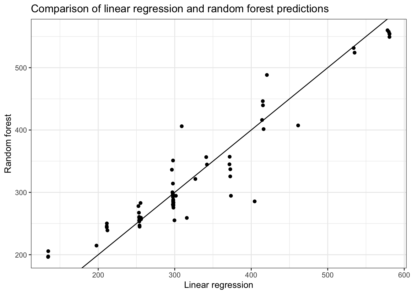
Let’s compare the predictions from the random forest model to the linear regression model:
Which seems very different to the lm() predictions.
References
A number of tags (including <p> and <li>) don’t require end tags, but I think it’s best to include them because it makes seeing the structure of the HTML a little easier.↩︎
This class comes from the xml2 package. xml2 is a low-level package that rvest builds on top of.↩︎